Post-processing
Path shortcutting
The paths found by the planning methods of Section Path planning are collision-free but might not be optimal in terms of path length. Some planning methods allow finding optimal paths, such as PRM* or RRT*, but they tend to be much slower and more difficult to implement compared to their non-optimal counterparts PRM and RRT. An efficient and widely-used approach consists in post-processing the paths found by PRM and RRT to improve the path quality. The algorithm below shows how to post-process a path by repeatedly applying shortcuts.
pseudo-code
'Algorithm: PATH_SHORTCUTTING
'Input: A collision-free path q
'Effect: Decrease the path length of q
FOR rep = 1 TO maxrep
  Pick two random points t1, t2 along the path
  IF the straight segment [q(t1),q(t2)] is collision-free THEN
    Replace original portion by the straight segment
Exercise: Post-processing a 2D path
Implement in Python the above algorithm to post-process the paths found in Section Path planning.
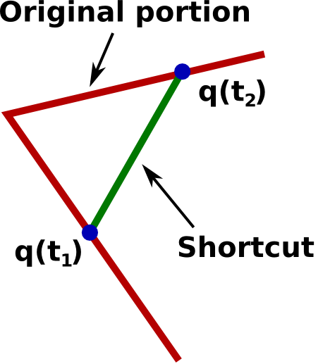
Trajectory shortcutting
The same idea as above can be applied to post-process trajectories. In trajectory planning, it is usually required to minimize trajectory duration.
pseudo-code
'Algorithm: TRAJECTORY_SHORTCUTTING
'Input: A valid trajectory q
'Effect: Decrease the trajectory duration of q
FOR rep = 1 TO maxrep
Pick two random points t1, t2 along the trajectory
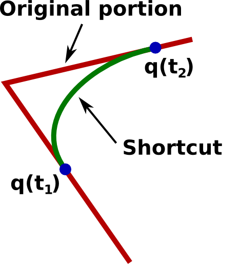
Generate a valid shortcut between q(t1) and q(t2) while ensuring velocity continuity
IF shortcut is collision-free AND has shorter time duration THEN
Replace original portion by shortcut
Note that
- "Valid" in the above algorithm means "being collision-free and respecting the kinodynamic constraints".
- Usually, in trajectory planning, it is required to ensure the continuity of the velocity, which can be achived as follows. The initial velocity of the shortcut must be equal to , and the final velocity of the shortcut must be equal to . Thus, the shortcut generation problem can be formulated as: find a curve starting from a given state and arriving at a given state , with minimal duration and subject to given kinodynamic constraints.
The next two sections present methods to generate such shortcut candidates, subject to (a) velocity and acceleration bounds, or (b) general second-order bounds.
Shortcutting with velocity and acceleration bounds
The problem here can be formulated as follows: given the start and goal states and , find a curve , such that , T is minimal and that
In the uni-dimensional case (N = 1), one can find the analytical expression for the time-optimal interpolant, which corresponds to a minimum time duration , see Hauser and Ng-Thow-Hing (2010). In the multi-dimensional case, one can compute the for each dimension i, and choose . Next, one can re-interpolate each dimension so that the time duration of each dimension is . One difficulty here is that the re-interpolation is not always possible. See Lertkultanon and Pham (2016) and https://github.com/Puttichai/parabint for an algorithm that can compute the re-interpolation for a large proportion of cases.
Shortcutting with general second-order bounds
For general second-order (kinodynamic) bounds, there are no analytical experession for time-optimal interpolants. One possible solution may consist in
- generating a smooth curve between and , without consideration of kinodynamic bounds;
- optimally time-parameterizing that curve (using the algorithm presented in Time-parameterization) so that it respects the kinodynamic bounds.
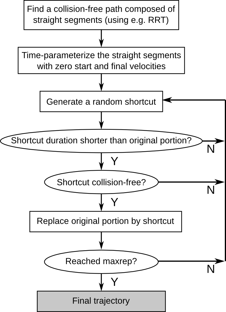
Complete motion planning pipeline
The following figure summarizes the complete motion pipeline as presented in this chapter. This pipeline is widely (if not the only one) used in motion planning software that are actually deployed on factory shop floors.
Complete motion planning pipeline in OpenRAVE
OpenRAVE's default planner actually follows exactly the pipeline just described. The following example shows how to use it on the scenario discussed at the beginning of this chapter.
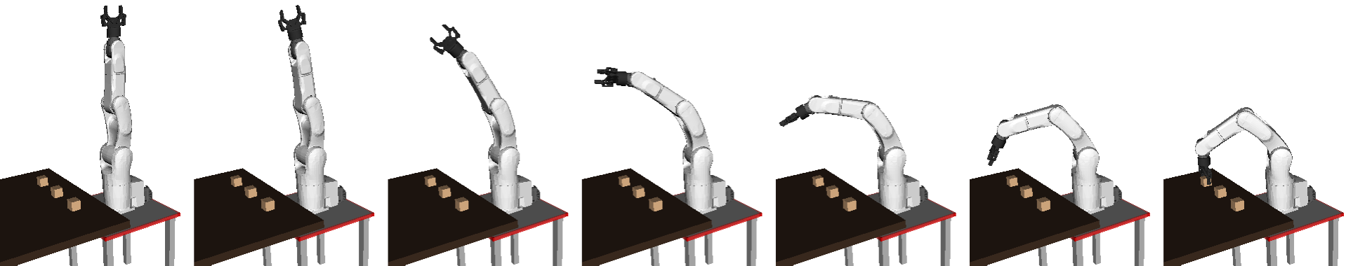
Example: Full motion planning pipeline in OpenRAVE
Here, we plan a fast, collision-free, motion from the robot initial configuration towards a configuration that allows grasping a box.
First, load the environment, the viewer and the robot (make sure that you have installed OpenRAVE, cloned the course repository, and changed directory to .
python
import numpy as np
import openravepy as orpy
env = orpy.Environment()
env.Load('osr_openrave/worlds/cubes_task.env.xml')
env.SetDefaultViewer()
robot = env.GetRobot('robot')
manipulator = robot.SetActiveManipulator('gripper')
robot.SetActiveDOFs(manipulator.GetArmIndices())
qgrasp = [-0.463648, 0.68088 , 1.477533, 0, 0.98318 , -2.034444]
The last line defines the grasping configuration, which was found using the IKFast solver (see Section Inverse kinematics). Now, we can use OpenRAVE's RRT planner
python
# Create the planner
planner = orpy.RaveCreatePlanner(env, 'birrt') # Using bidirectional RRT
params = orpy.Planner.PlannerParameters()
params.SetRobotActiveJoints(robot)
params.SetGoalConfig(qgrasp)
params.SetPostProcessing('ParabolicSmoother', '<_nmaxiterations>40</_nmaxiterations>')
planner.InitPlan(robot, params)
# Plan a trajectory
traj = orpy.RaveCreateTrajectory(env, '')
planner.PlanPath(traj)
# Execute the trajectory
controller = robot.GetController()
controller.SetPath(traj)
The function allows fine-tuning the post-processing, at both the path and trajectory levels. Here, we use parabolic shortcuts at the trajectory level () and repeat the shortcutting cycle 40 times (). Depending on applications, one can use other types of post-processing (e.g. linear shortcuts at the path level), increase the number of shortcutting cycles, etc.
To access the joint values along the trajectory, one can proceed as folows
python
times = np.arange(0, traj.GetDuration(), 0.01)
qvect = np.zeros((len(times), robot.GetActiveDOF()))
spec = traj.GetConfigurationSpecification()
for i in range(len(times)):
  trajdata = traj.Sample(times[i])
qvect[i,:] = spec.ExtractJointValues(trajdata, robot, manipulator.GetArmIndices(), 0)
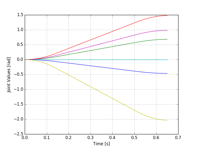
One can now plot the joint values
python
# Use the OO interface to avoid QT conflicts
from matplotlib.backends.backend_agg import FigureCanvasAgg as FigureCanvas
from matplotlib.figure import Figure
fig = Figure()
canvas = FigureCanvas(fig)
ax = fig.add_subplot(1,1,1)
ax.plot(times, qvect)
ax.grid(True)
ax.set_xlabel('Time [s]')
ax.set_ylabel('Joint Values [rad]')
canvas.print_figure('joint_values.png')
To learn more about this topic
Geraerts, R., & Overmars, M. H. (2007). Creating high-quality paths for motion planning. The International Journal of Robotics Research, 26(8), 845-863.
Hauser, K., & Ng-Thow-Hing, V. (2010). Fast smoothing of manipulator trajectories using optimal bounded-acceleration shortcuts. In Robotics and Automation (ICRA), 2010 IEEE International Conference on (pp. 2493-2498).
Pham, Q. C. (2015). Trajectory Planning. In Handbook of Manufacturing Engineering and Technology (pp. 1873-1887). Springer London.