Forward kinematics
Introductory example: a planar 2-DOF manipulator
Consider a planar manipulator with two revolute joints, as in the figure below. The joint angles are denoted by . The end-effector is a parallel gripper (in blue). The position and the orientation of the end-effector are denoted by . The forward kinematics problem is then to compute the mapping .
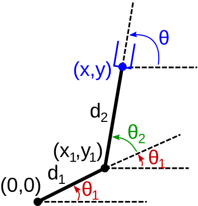
Applying simple trigonometry on the first link, one has
By similar calculations on the second link, one obtains
Finally, the orientation of the manipulator is given by .
One has thus obtained the explicit formulae for the forward kinematics function .
Jacobian matrix
Let us now introduce a fundamental object, the Jacobian matrix of the forward kinematics mapping.
Definition: Jacobian matrix
The Jacobian matrix of the forward kinematics mapping at a given configuration is defined by:
In the case of the planar 2-DOF manipulator, one has
Remarks:
- depends on the joint angles ;
- has as many columns as the number of joint angles (here: 2), and as many rows as the number of parameters of the end-effector (here: 3).
The Jacobian matrix is useful in that it gives the relationship between joint angle velocity and the end-effector velocity :
Exercise: FK in Python
Consider a planar 2-DOF manipulator as in the figure above, with the following dimensions .
Write the Python code of , which returns a triple representing the end-effector position and orientation for the joint angles
Write the Python code of , which returns a matrix representing the Jacobian matrix at
Assume that . Using the code just written, compute the values of:
What can you conclude?
Forward kinematics for 3D end-effectors
Transformation matrices
Usually, the end-effector is a rigid 3D object (rigid body). There are many ways to represent the orientations of rigid bodies: using e.g. Euler angles, quaternions, or rotation matrices. In this book, we shall use rotation matrices, which have many desirable properties. As a consequence, the positions/orientations of rigid bodies will be represented as transformation matrices, which are 4x4 matrices of the form
where is a 3x3 rotation matrix representing the orientation of the rigid body and is a vector of dimension 3 representing its position (or translation) in space. We shall also note .
More precisely, let us attach a rigid orthonormal frame to the rigid body, where is the origin of the body frame and are three orthonormal vectors. Then , , are the coordinates of respectively in the laboratory frame, and are the coordinates of in the laboratory frame.
The forward kinematics mapping is therefore, in the general case, .
Composition of transformations
As discussed above, transformation matrices can represent the position/orientation of a rigid body with respect to the (absolute) laboratory frame. They can also represent relative position/orientation between two rigid bodies (or two frames). In this case, one can denote for instance the transformation of frame B with respect by frame A by .
One can then compose transformations. Assume for instance that the end-effector (a gripper) is grasping a box. If the transformation of the end-effector with respect to the laboratory is given by and that of the box with respect to the end-effector is given by , then the transformation of the box with respect to the laboratory is given by
Rigid-body velocities
The velocity of a rigid body has two components: linear and angular. Consider again the orthonormal frame attached to the rigid body. In this case, the linear velocity is defined by the velocity of the point in the laboratory frame, that is
The angular velocity is defined by the velocity of the rotation of the vectors , which in turn can be represented by a vector of dimension 3. For instance, if the rigid body is rotating around a fixed axis, then the direction of is aligned with the axis of rotation and the norm of is the usual 2D angular velocity.
Given , the velocity in the laboratory frame of any point on the rigid body can be computed as
Relationship between rigid-body velocities and transformation matrices
Let us now clarify the relationship between (a) the above definitions of rigid-body velocities and (b) the transformation matrices that represent the positions/orientations of rigid bodies.
Assume that at time , the rigid body is at transformation , and that during a short amount of time , its linear and angular velocities are constant and equal to . Then, its transformation at time instant is given by:
where denotes the matrix exponential and denotes the matrix that represents a cross product with
Linear and angular Jacobians
Jacobian matrices for 3D end-effector can be defined in agreement with the above definitions of rigid-body velocities. Specifically, one can define the Jacobian for the linear velocity as the matrix that yields:
and the Jacobian for the angular velocity as the matrix that yields:
In practice, both matrices and can be computed from the robot structure.
Forward kinematics in OpenRAVE
Forward kinematics computations are efficiently implemented in OpenRAVE.
Transformation matrices
Example: FK in OpenRAVE (transformations)
First, load the environment, the viewer and the robot (make sure that you have installed OpenRAVE, cloned the course repository, and changed directory to .
python
import openravepy as orpy
env = orpy.Environment()
env.Load('osr_openrave/robots/denso_robotiq_85_gripper.robot.xml')
env.SetDefaultViewer()
robot = env.GetRobot('denso_robotiq_85_gripper')
manipulator = robot.SetActiveManipulator('gripper')
robot.SetActiveDOFs(manipulator.GetArmIndices())
Now, set the joint angles of the robot to the desired values and print out the manipulator transforms corresponding to those joint angle values.
python
robot.SetActiveDOFValues([0.1, 0.7, 1.5, -0.5, -0.8, -1.2])
print manipulator.GetEndEffectorTransform()
output
[[ 0.1017798  -0.43477328  0.89476984  0.63417832]
 [ 0.01692568  0.90006731  0.43542206  0.13759824]
 [-0.99466296 -0.02917258  0.0989675   0.43099054]
 [ 0.          0.          0.          1.        ]]
python
robot.SetActiveDOFValues([0.8, -0.4, 1.5, -0.5, -0.8, -1.2])
print manipulator.GetEndEffectorTransform()
output
[[ 0.64534243 -0.76378161 -0.01306916  0.09756635]
 [ 0.67405755  0.56131544  0.48017851  0.20609597]
 [-0.3594156  -0.31868893  0.87707343  0.95860823]
 [ 0.          0.          0.          1.        ]]
![OpenRAVE view at configuration [0.8, -0.4, 1.5, -0.5, -0.8,
-1.2].](../assets/kinematics/fk_openrave.png)
Note that the robot configuration in the viewer is updated in real time after each call.
Jacobian matrices
Example: FK in OpenRAVE (Jacobians)
First, load the environment, the viewer and the Denso robot
python
import openravepy as orpy
env = orpy.Environment()
env.Load('osr_openrave/robots/denso_robotiq_85_gripper.robot.xml')
env.SetDefaultViewer()
robot = env.GetRobot('denso_robotiq_85_gripper')
manipulator = robot.SetActiveManipulator('gripper')
robot.SetActiveDOFs(manipulator.GetArmIndices())
As the Jacobians depend on the joint angles, one must first set the joint angles of the robot to the desired values.
python
robot.SetActiveDOFValues([0.1, 0.7, 1.5, -0.5, -0.8, -1.2])
The linear Jacobian is computed by the function . This function has two arguments. The first argument is the link number of the end-effector. Here, assume that our end-effector is the base of the gripper. To determine the link number, one can use
python
robot.GetLinks()
output
[RaveGetEnvironment(1).GetKinBody('denso_robotiq_85_gripper').GetLink('link0'),
 RaveGetEnvironment(1).GetKinBody('denso_robotiq_85_gripper').GetLink('link1'),
 RaveGetEnvironment(1).GetKinBody('denso_robotiq_85_gripper').GetLink('link2'),
 RaveGetEnvironment(1).GetKinBody('denso_robotiq_85_gripper').GetLink('link3'),
 RaveGetEnvironment(1).GetKinBody('denso_robotiq_85_gripper').GetLink('link4'),
 RaveGetEnvironment(1).GetKinBody('denso_robotiq_85_gripper').GetLink('link5'),
 RaveGetEnvironment(1).GetKinBody('denso_robotiq_85_gripper').GetLink('link6'),
 RaveGetEnvironment(1).GetKinBody('denso_robotiq_85_gripper').GetLink('robotiq_coupler'),
 RaveGetEnvironment(1).GetKinBody('denso_robotiq_85_gripper').GetLink('robotiq_85_base_link'),
 RaveGetEnvironment(1).GetKinBody('denso_robotiq_85_gripper').GetLink('robotiq_85_left_knuckle_link'),
 RaveGetEnvironment(1).GetKinBody('denso_robotiq_85_gripper').GetLink('robotiq_85_right_knuckle_link'),
 RaveGetEnvironment(1).GetKinBody('denso_robotiq_85_gripper').GetLink('robotiq_85_left_finger_link'),
 RaveGetEnvironment(1).GetKinBody('denso_robotiq_85_gripper').GetLink('robotiq_85_right_finger_link'),
 RaveGetEnvironment(1).GetKinBody('denso_robotiq_85_gripper').GetLink('robotiq_85_left_inner_knuckle_link'),
 RaveGetEnvironment(1).GetKinBody('denso_robotiq_85_gripper').GetLink('robotiq_85_right_inner_knuckle_link'),
 RaveGetEnvironment(1).GetKinBody('denso_robotiq_85_gripper').GetLink('robotiq_85_left_finger_tip_link'),
 RaveGetEnvironment(1).GetKinBody('denso_robotiq_85_gripper').GetLink('robotiq_85_right_finger_tip_link')]
Thus, the gripper base link () is link number 8.
The second argument of is the position in the laboratory frame of the reference point on the rigid body we mentioned previously. One can choose to be for instance the origin of the link frame.
Putting everything together, we obtain the following code
python
link_idx = [l.GetName() for l in robot.GetLinks()].index('robotiq_85_base_link')
link_origin = robot.GetLink('robotiq_85_base_link').GetTransform()[:3,3]
# Improve the visualization settings
import numpy as np
np.set_printoptions(precision=6, suppress=True)
# Print the result
print robot.ComputeJacobianTranslation(link_idx, link_origin)
output
[[-0.076639  0.071775 -0.160337  0.019553  0.018678 -0.        0.      ]
 [ 0.508911  0.007201 -0.016087 -0.044858 -0.022967  0.        0.      ]
 [ 0.       -0.514019 -0.317533  0.020576 -0.067821 -0.        0.      ]]
The angular Jacobian is computed by the function . This function has one argument: the link number of the end-effector.
python
print robot.ComputeJacobianAxisAngle(link_idx)
output
[[ 0.       -0.099833 -0.099833  0.804457 -0.368345  0.89477   0.      ]
 [-0.        0.995004  0.995004  0.080715  0.845031  0.435422  0.      ]
 [ 1.        0.        0.       -0.588501 -0.387614  0.098967  0.      ]]
Exercise
Exercise: FK in OpenRAVE
Consider the same Denso robot as previously. Assume that at time , we have:
Questions:
- Compute the transformation matrix of the at configurations and .
- Compute the linear and angular Jacobians of the at time .
- Using these Jacobians, compute another approximation of the transformation matrix of the at time .
To learn more about this topic
See Chapters 4 and 5 of
Lynch, K. M., & Park, F. C. (2017). Modern Robotics: Mechanics, Planning, and Control. Cambridge University Press. Available at http://modernrobotics.org