Path planning
There exists a large variety of approaches to path planning: combinatorial methods, potential field methods, sampling-based methods, etc. Sampling-based methods are the most efficient and robust, hence probably the most widely used for path planning in practice. Sampling-based methods include Grid Search, Probabilistic Roadmap (PRM) and Rapidly-exploring Random Trees (RRT), which are presented in the next two sections.
Grid Search and Probabilistic Roadmap (PRM)
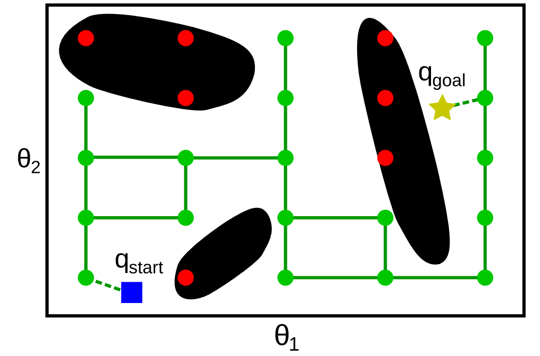
A first category of sampling-based methods requires building, in a preprocessing stage, a roadmap that captures the connectivity of . A roadmap is a graph G whose vertices are configurations of . Two vertices are connected in G only if it is possible to connect the two configurations by a path entirely contained in . Once such a roadmap is built, it is easy to answer the path planning problem: if
- can be connected to a (nearby) vertex u;
- can be connected to a (nearby) vertex v;
- u and v are in the same connected component of G (in the graph-theoretic sense),
then there exists a collision-free path between and (see figure below).
Methods for building the roadmap fall into two families: deterministic or probabilistic. A typical deterministic method is the Grid Search, where the configuration space is sampled following a regular grid, as in the figure below. A sampled configuration is rejected if it is not in . Next, one attempts to connect every pair of adjacent configurations (adjacent in the sense of the grid structure) to each other: if the straight segment connecting the two configurations is contained within , then the corresponding edge is added to the graph G.
To check whether a segment is contained within , one may sample many points along the segment and check whether all those points are in .
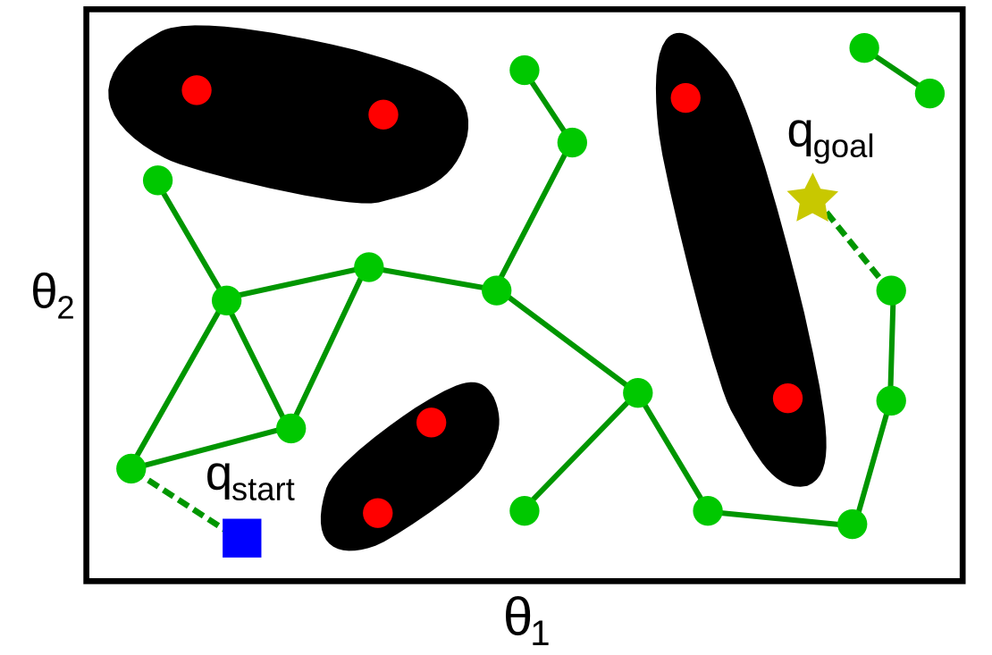
In the Probabilistic Roadmap method, instead of following a regular grid, samples are taken at random in , see figure below. Since there is no a priori grid structure, several methods exist for choosing the pairs of vertices for which connection is attempted: for instance, one may attempt, for each vertex, to connect it to every vertices that are within a specified radius r from it.
Strengths of roadmap-based methods
The strength of the roadmap-based methods (both deterministic and probabilistic) comes from the global/local decomposition – the difficult problem of path planning is solved at two scales: the local scale, where neighboring configurations (adjacent configurations in Grid Search, configurations within a small distance r of each other in the Probabilistic Roadmap) are connected by a simple straight segment; and the global scale, where the graph search takes care of the global, complex connectivity of the free space.
Note also that it is not necessary for these methods to have an explicit representation of : one only needs an oracle which says whether a given configuration is in . To check whether a straight segment is contained within , it suffices to call the oracle on every configuration (or, in practice, on sufficiently densely sampled configurations) along that segment.
These methods also possess nice theoretical guarantees. Specifically, it can be shown that the Grid Search is resolution complete, which means that if a solution exists, the algorithm will find it in finite time and for a sufficiently small grid size. Similarly, it can be shown that the Probabilistic Roadmap method is probabilistically complete, which means that, if a solution exists, the probability that the algorithm will find it converges to 1 as the number of sample points goes to infinity. However, the converge rate of both methods is difficult to determine on practical problem instances.
Regarding the comparative performances of the deterministic and probabilistic approaches, it has been shown both theoretically and practically that randomness is not advantageous in terms of search time. However, it can be argued that probabilistic methods are easier to implement.
Exercise: Solving a 2D motion planning problem by PRM
First, load a simple 2D environment (make sure that you have cloned the course repository, and changed directory to .
python
import numpy as np
import pylab as pl
import sys
sys.path.append('osr_examples/scripts/')
import environment_2d
pl.ion()
np.random.seed(4)
env = environment_2d.Environment(10, 6, 5)
pl.clf()
env.plot()
q = env.random_query()
if q is not None:
  x_start, y_start, x_goal, y_goal = q
  env.plot_query(x_start, y_start, x_goal, y_goal)
This should generate an environment as follows
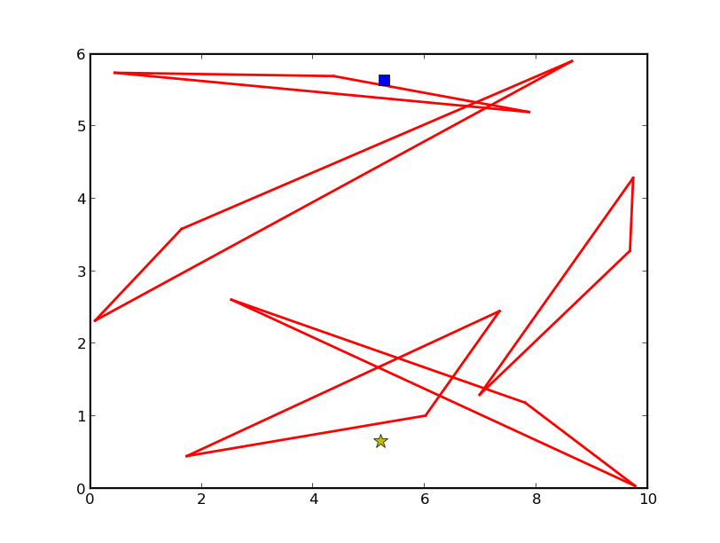
Question: Implement the PRM algorithm described earlier to solve this problem instance. Generate other query instances and environment instances and test your algorithm.
Hint: you may use the function , which returns if the point is contained within a triangular obstacles, otherwise.
Rapidly-exploring Random Trees (RRT)
The methods just discussed require building the entire roadmap in the preprocessing stage before being able to answer any query [a query being a pair (, ) to be connected]. In applications where only a single or a limited number of queries are needed, it may not be worthy to build the whole roadmap. Single-query methods, such as the Rapidly-exploring Random Trees (RRT), are much more suited for these applications.
Specifically, RRT iteratively builds a tree (see Algorithm 1), which is
also a roadmap, but which has the property of exploring “optimally” the
free space. The key lies in the EXTEND{.sourceCode} function, which
selects the vertex in the tree that is the closest to the randomly
sampled configuration (see Algorithm 2). Thus, the
probability for a vertex in the tree to be selected is proportional to
the size of its Voronoi region, causing the tree to grow preferably
towards previously under-explored regions.
pseudo-code
'Algorithm: BUILD_RRT
'Input: A starting configuration q_start
'Output: A tree T rooted at q_start
T.INITIALIZE(q_start)
FOR rep = 1 TO maxrep
  q_rand ← RANDOM_CONFIG()
  EXTEND(T, q_rand)
pseudo-code
'Algorithm: EXTEND
'Input: A tree T and a target configuration q_rand
'Effect: Grow T by a new vertex in the direction of q_rand
q_near ← NEAREST_NEIGHBOR(T, q_rand)
IF q_new ← STEER(q_near, q_rand) succeeds THEN
  T.ADD_VERTEX(q_new)
  T.ADD_EDGE([q_near, q_new])
Note: attempts making a straight motion from towards . Three cases can happen
- is within a given distance of and is collision-free, then is returned as the new vertex ;
- is farther than a given distance of , and the segment of length from and in the direction of is collision-free, then the end of that segment is returned as (see figure below);
- else, returns .

Finally, to find a path connecting and , one can grow simultaneously two RRTs, one rooted at and the other rooted at , and attempt to connect the two trees at each iteration. This algorithm is known as bidirectional RRT. In practice, bidirectional RRT has proved to be easy to implement, yet extremely efficient and robust: it has been successfully applied to a large variety of robots and challenging environments.
Exercise: Solving a 2D motion planning problem by RRT
Implement the RRT algorithm to solve the problem instance of the PRM exercise above. Generate other query instances and environment instances and test your algorithm. Compare the running times of RRT and PRM on single and multiple queries problem instances.
To learn more about this topic
See Chapters 5 and 6 of
LaValle, S. M. (2006). Planning algorithms. Cambridge University Press. Available at http://planning.cs.uiuc.edu