Motion planning
Consider the task discussed in the Overview of this course: “pick up an object from the tabletop”.
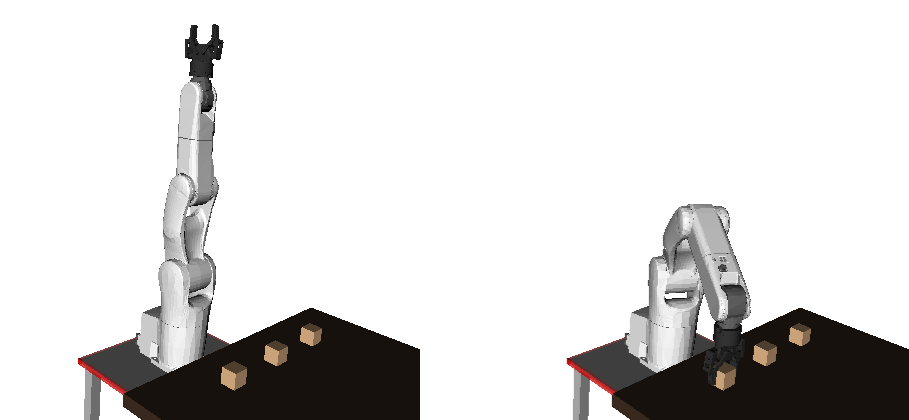
To properly grasp the object, the gripper must be placed in a particular position and orientation , such as in the right figure above. In Section [Inverse kinematics], we presented algorithms to find the joint angles that achieves the desired gripper position and orientation.
The motion planning problem consists in finding the appropriate robot commands to move the robot from the starting joint angle configuration towards the desired goal configuration , while satisfying the following requirements
avoid collisions between the robot and the environment (the table, the object to be grasped) or with itself (self-collision) [geometric or configuration-space constraints];
respect the robot kinematics and dynamics (kinodynamic) constraints, such as bounds on joint velocities, accelerations, or torques [kinodynamic or state-space constraints];
minimize some criteria, such as execution time or energy consumption.
We have seen in Section Inverse kinematics that the configuration space of the manipulator is the set of all possible joint angle values . Before proceeding further, we need some definitions.
Definition: Obstacle and free configuration space
The subset of that consists of joint angles values where the robot collides with the environment or with itself is called the obstacle space and denoted . The complement of is called the free space and denoted .
Definition: Path, time-parameterization, trajectory
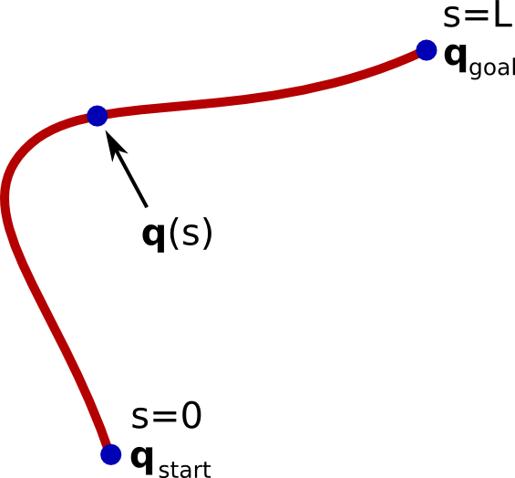
Formally, a path in the configuration space can be defined as the image of a continuous function P where
A path can be regarded as a geometric object devoid of any timing information. By abuse of notation, we shall refer to as the path. Next, a time-parameterization of is a strictly increasing function
with and . The function gives the position on the path for each time instant . The path endowed with a time-parameterization becomes a trajectory
with being the duration of the trajectory. Note that the same path can give rise to many different trajectories .
To solve the motion planning problem, we shall adopt the decoupled planning approach: first plan a collision-free path that satisfies the geometric constraints (i.e. a path entirely contained in ). Second, find a time-parameterization of that path to satisfy the kinodynamic constraints, while minimizing execution time. This pipeline has been found to be the most robust and efficient motion planning approach, and is therefore widely used in actual industrial applications. Other approaches, which consists e.g. in planning directly in the state-space (i.e. the space of joint angles and joint velocities), have some nice theoretical properties but are rarely use in practice.
In Section Path planning, we discuss methods to find a collision-free path between and .
In Section Time parameterization, we present methods to find the time-stamps for the joint angles along the path, so as to satisfy bounds on velocity, acceleration or torques while optimizing execution time.
In Section Post-processing, we study some methods to further improve the quality of trajectories found in the previous steps, in terms of execution time or trajectory smoothness.