Inverse kinematics
Introductory example: a planar 2-DOF manipulator
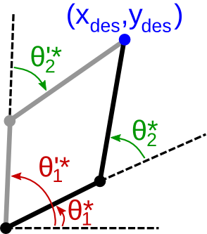
Consider the same planar 2-DOF manipulator as in Section Forward kinematics. Suppose that we want to place the gripper at a desired position (the gripper orientation does not matter for now). Finding the appropriate joint angles that achieve this position constitutes the inverse kinematics problem.
Recall that
Squaring both sides of the equations and adding them together yield:
Thus,
There are two cases:
- If , then there are no solutions. Intuitively, this means that the desired position for the end-effector is too far away to be reached;
- Else, there are two solutions for :
Next, after some calculations, one can find the expression of as:
where:
The above derivations raise the following remarks:
- Inverse kinematics calculations are in general much more difficult than forward kinematics calculations;
- While a configuration always yields one forward kinematics solution , a given desired end-effector position may correspond to zero, one, or multiple possible IK solutions .
Exercise: IK in Python
Consider a planar 2-DOF manipulator as in the figure above, with the following dimensions .
- Write the Python code for ;
- Execute and . Your code should return respectively 2 and 0 solutions.
Inverse kinematics for robot manipulators
Dimensions of the configuration space and of the task space
Definition: Configuration space
In the general case, the set of all possible robot joint angles will be refered to as the configuration space of the robot and denoted . The dimension of the configuration space is then the number of robot joints, which is 6 in the case of the Denso manipulator considered in this book.
Definition: Task space
The task space is defined with respect to the task at hand. Consider for instance a grasping task. To properly grasp an object, the end-effector must be placed in a precise 3D position and 3D orientation. In this case, the task space is the set of all desired 3D positions/orientations, which has dimension 6 (3 position coordinates and 3 orientation coordinates). Consider now a drilling task. Here, one needs to place the tip of the drill bit at the desired hole position (3 position coordinates) and to ensure that the drill bit is perpendicular to the drilled surface (2 orientation coordinates: the rotation around the surface normal is irrelevant), yielding a task space of dimension 5.
In general, the dimension of the configuration space must be larger or equal to the dimension of the task space to ensure the existence of IK solutions for a significant proportion of desired task values.
Redundancy
Redundancy arises when there are multiple IK solutions for a given desired task value. Consider the planar 2-DOF manipulator as above. For the given value of the task, there are two distinct IK solutions, namely and . For a manipulator with 6 revolute joints (such as our Denso robot) and a 6D task (position and orientation of the end-effector), there can exist up to 16 distinct IK solutions for a given desired position/orientation of the end-effector. This type of redundancy, when the configuration space and the task space has the same dimension, can be termed discrete redundancy.
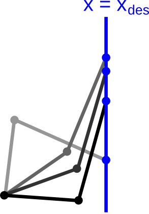
Redundancy is more prominent when the dimension of the configuration space is strictly larger than the dimension of the task space. Consider again the planar 2-DOF manipulator, but assume now that the task is to place the gripper on a vertical line — the vertical coordinate and the gripper orientation do not matter. In this case, the task space has dimension 1 (desired values for ), and there are an infinite number of IK solutions for each desired value of . This type of redundancy can be termed continuous redundancy.
IK computations
Task-space analytical IK
We have seen in the IK derivations for a planar 2-DOF manipulator that the equations are quite complex, involving multiple inverse trigonometric functions and validity conditions. For general 6-DOF manipulators and 6D task spaces, which constitute the most common use of IK, the equations are even more difficult, and there are in general no closed-form formulae.
Velocity-space (or differential) IK
Up to know, we have considered the “task-space” IK problem, that is, given a desired task value , find the configuration so that . This problem is very difficult since is in general a complex, nonlinear, function, which is difficult to invert.
Consider now the “velocity-space” (or “differential”) IK problem: suppose that the robot is at a configuration , what joint angle velocity will achieve a given a desired task-space velocity (for example, we would like the end-effector to move with some desired linear and angular velocities)?
This problem is much more tractable than the “task-space IK” problem. Indeed, from Section Forward kinematics, we know that
which is a linear mapping between and .
Thus, if the dimensions of the configuration space and task space are equal (which implies that the Jacobian matrix is square) and that the Jacobian matrix is invertible, then is simply given by
If the Jacobian matrix is not invertible, then is called a singular configuration, and should be avoided when doing velocity-space IK.
If the dimensions of the configuration space is strictly larger than the dimension of the task space (redundant case), then the linear equation
has multiple solutions . In such a case, one may choose to optimize some other criteria. For instance, if one is interested in the smallest joint angle velocity, then one may choose
where is the pseudo-inverse of .
Task-space IK using velocity-space IK
One can use velocity-space IK to find approximate task-space IK solutions as follows
- Start from an arbitrary configuration and compute the forward kinematics ;
- Choose a path in the task space between and , for instance a straight line;
- Divide that path into small chunks with ;
Using velocity-space IK, compute iteratively:
If the path chunks are small enough, then one should have .
The above scheme is easy to implement but has some drawbacks:
- For good approximation accuracy, one may need to divide the task-space path into many small chunks, which increases computation time;
- The scheme fails if the path goes near a singularity in the configuration space;
- In the discrete redundancy case, this scheme can, in general, only generate one task-space IK solution;
- The choice of the initial configuration affects the IK solution that is eventually found.
Inverse kinematics in OpenRAVE
Task-space analytical IK: IKFast
As mentioned previously, there is in general no closed-form formulae for task-space analytical IK. Thus, most of existing IK solvers are based on the velocity-space IK scheme just presented. The IK solver implemented in OpenRAVE, IKFast, takes a different approach. Given a robot kinematic model, IKFast automatically generates, in an offline stage, a program that can compute numerical task-space IK solutions. This program generation can take up to several minutes. At runtime, given a desired task value , the program will be executed on this value, and computation times at this stage are extremely fast. The advantages of IKFast are
- It is fast and accurate (several magnitude faster than velocity-space IK schemes);
- In the discrete redundancy case, it can give all IK solutions, not just one. This is particularly important since choosing a “good” IK solution can dramatically simplify the subsequent motion planning problem.
Example: 6D IK with OpenRAVE’s IKFast
First, load the environment, the viewer and the robot (make sure that you have installed OpenRAVE, cloned the course repository, and changed directory to .
python
import numpy as np
import openravepy as orpy
import tf.transformations as tr
env = orpy.Environment()
env.Load('osr_openrave/worlds/cubes_task.env.xml')
env.SetDefaultViewer()
robot = env.GetRobot('robot')
manipulator = robot.SetActiveManipulator('gripper')
robot.SetActiveDOFs(manipulator.GetArmIndices())
np.set_printoptions(precision=6, suppress=True)
# Box to illustrate elbow up/down
with env:
  box = orpy.RaveCreateKinBody(env, '')
  box.SetName('box')
  box.InitFromBoxes(np.array([[0.5, 0.3, 1, 0.01, 0.04, 0.22]]), True)
  env.AddKinBody(box)
To grasp the red box on the table, one needs to move the gripper towards the following position
python
box_centroid = box.ComputeAABB().pos()
print box_centroid
output
[ 0.5 0.3 1.]
For this, one can do as follows
python
ikmodel = orpy.databases.inversekinematics.InverseKinematicsModel(robot, iktype=orpy.IkParameterization.Type.Transform6D)
if not ikmodel.load():
  ikmodel.autogenerate()
Tgrasp = tr.quaternion_matrix([ 0.5,  0.5,  0.5, -0.5])
Tgrasp[:3,3] = box_centroid
solutions = manipulator.FindIKSolutions(Tgrasp, 0)
print solutions
output
[[ 0.170333  2.002192 -1.09442   4.606915 -1.436798 -2.471484]
 [ 0.170333  0.884552  1.161062 -1.492324 -1.41946   2.660823]
 [ 0.170333  0.884552  1.161062 -4.633916  1.41946  -0.48077 ]
 [ 0.170333  2.002192 -1.09442   1.465323  1.436798  0.670108]
 [ 0.170333  0.884552  1.161062  1.649269  1.41946  -0.48077 ]
 [ 0.170333  2.002192 -1.09442  -1.67627  -1.436798 -2.471484]]
The first four lines initialize the IK solver and set the desired manipulator transform . Next, the IK solver is called by , which takes two arguments. The first argument is the desired manipulator transform. The second argument is a flag that filters the solutions. A flag value of 0 makes the algorithm return all solutions. Here, one can see that there are six possible solutions.
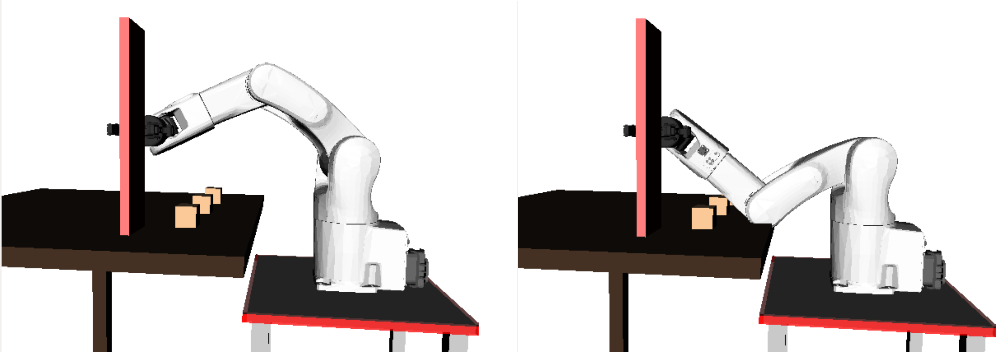
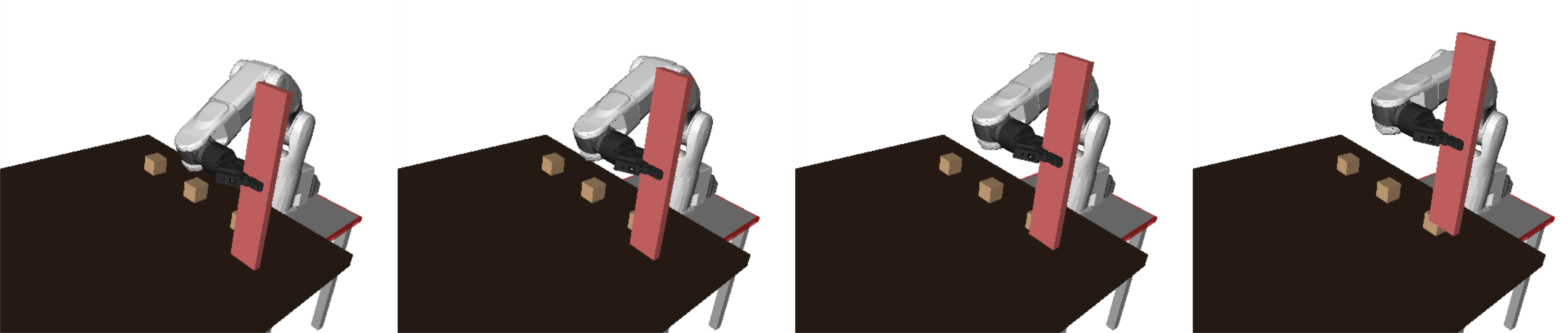
To check out, for example, solutions number 4 and number 0, one can do (see figure below)
python
robot.SetActiveDOFValues(solutions[4])
robot.SetActiveDOFValues(solutions[0])
If one wishes to consider only IK solutions that are collision-free, one can use
python
solutions = manipulator.FindIKSolutions(Tgrasp, orpy.IkFilterOptions.CheckEnvCollisions)
print solutions
output
[[ 0.170333  0.884552  1.161062  1.649269  1.41946  -0.48077 ]
 [ 0.170333  0.884552  1.161062 -1.492324 -1.41946   2.660823]
 [ 0.170333  0.884552  1.161062 -4.633916  1.41946  -0.48077 ]]
Velocity-space IK
Example: Velocity-space IK with OpenRAVE
Velocity-space (or differential) IK is typically used to continuously move the manipulator following some task-space constraints. Consider the scenario in the previous example, where the object has been grasped. Suppose that we would like to move the object upwards by 10 cm, without changing its orientation. This can be achieved by constraining the translation velocity of the manipulator to be aligned with the Z-axis and the rotation velocity of the manipulator to be 0.
First, load the environment and set the robot to the grasping configuration
python
import numpy as np
import openravepy as orpy

env = orpy.Environment()
env.Load('worlds/cubes_task.env.xml')
env.SetDefaultViewer()
robot = env.GetRobot('robot')
manipulator = robot.SetActiveManipulator('gripper')
robot.SetActiveDOFs(manipulator.GetArmIndices())
np.set_printoptions(precision=6, suppress=True)
# Working box
with env:
  box = orpy.RaveCreateKinBody(env, '')
  box.SetName('box')
  box.InitFromBoxes(np.array([[0.5, 0.3, 1, 0.01, 0.04, 0.22]]), True)
  env.AddKinBody(box)

qgrasp = [0.170333, 0.884552, 1.161062, 1.649269, 1.41946, -0.48077 ]
robot.SetActiveDOFValues(qgrasp)
# Close the gripper and grab the box
taskmanip = orpy.interfaces.TaskManipulation(robot)
taskmanip.CloseFingers()
robot.WaitForController(0)
robot.Grab(box)
The last command makes the box stick to the end-effector of the robot, mimicking a grasping behavior.
Consider now the following 6D velocity vector
python
twist = np.array([0, 0, 0.01, 0, 0, 0])
The first three coordinates are the desired translation in each step, which is 0 in X, 0 in Y and 1 cm in Z. The last three coordinates are the desired rotation in each step, which is 0.
We can now perform the differential IK as follows
python
link_idx = [l.GetName() for l in robot.GetLinks()].index('robotiq_85_base_link')
link_origin = robot.GetLink('robotiq_85_base_link').GetTransform()[:3,3]
J = np.zeros((6,6))
q = robot.GetActiveDOFValues()
for i in range(10):
  J[:3,:] = robot.ComputeJacobianTranslation(link_idx, link_origin)[:,:6]
  J[3:,:] = robot.ComputeJacobianAxisAngle(link_idx)[:,:6]
  qdot = np.linalg.solve(J, twist)
  q[:6] += qdot
  robot.SetDOFValues(q)
  raw_input('Press Enter for next differential IK step')
Exercise: Task-space IK using velocity-space IK
Implement the scheme described in section “Task-space IK using velocity-space IK” and compare with IK Fast in terms of
- computation time;
- accuracy of the IK solution.
To learn more about this topic
See Chapter 6 of
Lynch, K. M., & Park, F. C. (2017). Modern Robotics: Mechanics, Planning, and Control. Cambridge University Press. Available at http://modernrobotics.org